Building a LinkedIn Analytics Pipeline on Databricks — Part 3: Building the Medallion Pipeline

Part 3 of 4 of the Series on getting LinkedIn data into Databricks

This is the third post in a four-part series. Part 1 set up the project scaffold. Part 2 covered connecting to the LinkedIn API and landing raw JSON in a Databricks Volume. Part 4 covers creating a dashboard and cost of running this pipeline.

In Part 2, the ingest notebook ran and five directories of JSON files appeared in the landing volume. Raw, nested, unprocessed: one file per API call, each containing a list of daily data points buried inside an elements array.

Now we transform that into something queryable. A single daily_metrics table, one row per day, all five metrics as columns, deduplicated and ready for a dashboard.

This is what Declarative Pipelines is built for.

The medallion architecture, briefly

The pipeline follows the medallion pattern: Bronze → Silver → Gold. Each layer has a distinct purpose.

Bronze is faithful to the source. It reads raw files as-is and adds just enough metadata to make the data traceable, e.g. a file path and an ingestion timestamp. No business logic, no transformations that could lose information.

Silver is clean and keyed. It takes the raw bronze data and produces deduplicated, typed tables with one row per date per metric. This is where duplicates are resolved and where late-arriving data gets handled correctly.

Gold is analytics-ready. It joins all the silver tables into a single wide table that’s trivial to query from a dashboard or notebook.

The whole pipeline is defined in three SQL files and wired together by a single Declarative Pipelines configuration.

Building the Pipeline

Setting things up in Declarative Automation Bundles

We will set up a Spark Declarative Pipeline using Declarative Automation Bundles. I am not sure if Databricks did a good job in the renaming at the beginning of 2026. It definitely confuses me sometimes and adds mental load to untangle the declarative stuff.

In Part 1 we set up the basic repo structure. Now, we will add pipelines.yml to the resources folder. This defines the basic parameters of the pipeline we are about to create.

resources:
  pipelines:
    linkedin_transform:
      name: linkedin-transform
      catalog: ${var.catalog}
      schema: ${resources.schemas.bronze_linkedin.name}
      serverless: true
      channel: CURRENT
      continuous: false
      configuration:
        volume: /Volumes/${var.catalog}/${resources.schemas.bronze_linkedin.name}/${resources.volumes.landing.name}
        silver_schema: ${var.catalog}.${resources.schemas.silver_linkedin.name}
        gold_schema: ${var.catalog}.${resources.schemas.gold_linkedin.name}
      libraries:
        - file:
            path: ../src/pipelines/load_bronze.sql
        - file:
            path: ../src/pipelines/load_silver.sql
        - file:
            path: ../src/pipelines/load_gold.sql
      run_as:
        service_principal_name: ${var.service_principal_app_id}

      tags:
        project: linkedin

This pipeline is running on serverless. This is optimal since we expect it to finish very quickly (1-2 minutes) so we can spare ourselves the startup time of a classic compute instance that takes about 5 minutes.

The pipeline references load_bronze.sql, load_silver.sql and load_gold.sql as so-called libraries. We will find out what will be in these files in the next section.

Bronze: reading JSON as streaming tables

Back to our business case. In Part 2 we downloaded the LinkedIn metrics into JSON files and stored them in a Volume. Now it is time to read them into bronze tables. The read_files function handles this cleanly with a STREAM source, which means Declarative Pipelines tracks which files have already been processed and only picks up new ones on each run.

CREATE OR REFRESH STREAMING TABLE impressions
COMMENT “Raw post impression data ingested from the LinkedIn API landing volume”
AS SELECT
    *,
    CURRENT_TIMESTAMP() AS _timestamp,
    _metadata.file_path AS _filename
FROM
    STREAM read_files(
        “${volume}/impressions/”,
        format => “json”
    );

Two things worth noting here.

First, _metadata.file_path is a hidden column that Spark populates automatically when reading files. It gives you the full path of the source file for each row. I capture it as _filename and carry it all the way through to silver, where it becomes the sequencing key for CDC. More on that shortly.

Second, ${volume} is the pipeline configuration variable resolved at runtime from the bundle and contains the full path to the Databricks Volume. This keeps the SQL environment-agnostic; the same code runs in dev and prod pointing at different catalogs.

Each raw table is one row per file. But LinkedIn’s API returns each metric as a list of daily data points nested inside an elements array. To get to one row per day, each raw table needs to be exploded.

CREATE OR REFRESH STREAMING TABLE impressions_exploded
AS SELECT
    MAKE_DATE(element.dateRange.start.year,
              element.dateRange.start.month,
              element.dateRange.start.day) AS date,
    element.count AS count,
    _timestamp,
    _filename
FROM (
  SELECT
        EXPLODE(elements) AS element,
        _timestamp,
        _filename
  FROM STREAM(impressions)
  WHERE elements IS NOT NULL
);

The MAKE_DATE call converts LinkedIn’s year/month/day struct into a proper SQL DATE. The WHERE elements IS NOT NULL filter drops any files that contain an API error response. As covered in Part 2, LinkedIn can return HTTP 200 with an error body that has no elements field. Rather than letting those rows corrupt the pipeline, we skip them at the bronze layer.

The Followers Count problem: when there’s no date in the response

Four of the five API endpoints return data with an explicit dateRange per element, so deriving the date is straightforward. The fifth, memberFollowersCount?q=me, which returns your current total follower count, doesn’t. It’s a point-in-time snapshot with no temporal context in the response body.

The solution is to derive the date from the filename itself. Because the ingest notebook writes files with a 14-digit timestamp in the name (followers_agg_20260315060114.json), that timestamp tells us exactly when the snapshot was taken.

CREATE OR REFRESH STREAMING TABLE followers_agg_exploded
AS SELECT
    TO_DATE(file_datetime) AS date,
    element.memberFollowersCount AS count,
    _timestamp,
    _filename
FROM (
    SELECT
        EXPLODE(elements) AS element,
        to_timestamp(
            regexp_extract(_filename, r’(\d{14})\.json$’, 1),
            ‘yyyyMMddHHmmss’
        ) AS file_datetime,
        _timestamp,
        _filename
    FROM STREAM(followers_agg)
    WHERE elements IS NOT NULL
);

regexp_extract pulls the 14-digit sequence from the filename, to_timestamp parses it using the yyyyMMddHHmmss format, and TO_DATE truncates to the day. This is why the filename timestamp convention in the ingest notebook matters — it’s not just cosmetic, it’s load-bearing.

A purist reading of the medallion architecture would push back on the above approach: Bronze should be a faithful copy of the source, nothing more. Exploding an array changes the row count and the schema: that’s a transformation, and transformations belong in Silver.

It’s a fair point. But I made a deliberate choice to keep a two-table pattern within Bronze: one raw table (one row per file, exactly as the API returned it) and one exploded table derived from it. The raw table is never modified. If the LinkedIn API changes its response shape tomorrow, the original payload is still there to re-process. The explosion is light structural preparation, not business logic, and keeping it in Bronze means Silver has exactly one job: deduplication. The CDC upsert logic is cleaner when it receives already-flat, already-typed rows.

The Followers Count date derivation that is extracting the snapshot date from the filename sits in the same category. Strictly speaking it’s a transformation; pragmatically, it belongs close to the source where the context (the filename convention) is most visible.

This is a tradeoff worth being conscious of, not a rule violation. If the pipeline grew significantly in complexity, pushing the explosion into Silver would be the right call. But this would cause some headaches, such as the fact that Auto CDC requires a streaming table as input. At this scale, keeping Bronze slightly wider than the strict definition earns simplicity elsewhere.

Silver: CDC upserts for idempotent daily records

The bronze exploded tables are append-only streaming tables. Every time the pipeline runs, new rows flow in. For the delta load (rolling 60-day window), that means the same dates arrive repeatedly. Monday’s run includes data for the last 60 days, Tuesday’s run includes the same 59 days plus one new one. Without deduplication, the silver tables would accumulate duplicates fast. Additionally, that would not make sense from an analytical perspective.

Declarative Pipelines’ AUTO CDC feature handles this with a MERGE-based CDC flow. You declare a target table, tell it what the key is, and the pipeline handles the upsert logic:

CREATE OR REFRESH STREAMING TABLE ${silver_schema}.impressions
  (date    DATE    COMMENT “Calendar date of the impression data point”,
   count   BIGINT  COMMENT “Number of post impressions on this date”)
COMMENT “Deduplicated daily post impression counts, keyed by date (SCD Type 1)”;
CREATE FLOW impressions_cdc_flow
AS AUTO CDC INTO ${silver_schema}.impressions
FROM STREAM(impressions_exploded)
KEYS (date)
SEQUENCE BY _filename
COLUMNS * EXCEPT (_filename, _timestamp)
STORED AS SCD TYPE 1;

A few things to unpack here.

• KEYS (date) means each date is a unique record. If the same date arrives again (because of a re-run or an overlapping delta window), it’s treated as an update, not a new row.

• SEQUENCE BY _filename is the ordering mechanism. Declarative Pipelines needs to know which version of a record “wins” when the same key arrives multiple times. Using the filename (which contains a timestamp) means a file written by a later run will always supersede one written by an earlier run. The pipeline is idempotent: re-running it won’t corrupt the data, it will just update records to their latest values.

• STORED AS SCD TYPE 1 means we overwrite. No history is kept when a value changes. For this use case, LinkedIn’s API can revise recent metrics slightly after the fact, and I want the silver layer to always reflect the most current values LinkedIn returns, not accumulate a change log.

• COLUMNS * EXCEPT (_filename, _timestamp) means the internal pipeline metadata columns don’t land in the silver table. Only date and count are written to the target.

The same pattern repeats for all five metrics: followers, followers_agg, impressions, reactions, comments. Each gets a target table declaration and a CDC flow.

All of this goes into the load_silver.sql file in the src/pipelines folder.

Gold: one wide table with a UNION spine

The silver layer gives us five clean tables, each with a date column and a count column. The gold layer joins them into a single daily_metrics table with one row per date, all five metrics as named columns.

The tricky part is that not every metric has a value for every date. On a day with no posts, reactions and comments might be zero or absent entirely. A naive join using any one table as the spine would silently drop dates that exist in other tables.

The solution is a UNION spine: take all distinct dates from all five tables, use that as the base, and LEFT JOIN each metric onto it.

This code goes into the load_gold.sql file in the src/pipelines folder:

CREATE OR REFRESH MATERIALIZED VIEW ${gold_schema}.daily_metrics
  (date                   DATE    COMMENT “Calendar date of the metrics”,
   followers_delta_count  BIGINT  COMMENT “Net change in followers on this date”,
   followers_count        BIGINT  COMMENT “Total follower count snapshot on this date”,
   impressions_count      BIGINT  COMMENT “Number of post impressions on this date”,
   reactions_count        BIGINT  COMMENT “Number of post reactions on this date”,
   comments_count         BIGINT  COMMENT “Number of post comments on this date”)
COMMENT “LinkedIn daily metrics combining followers, impressions, reactions, and comments”
AS
WITH all_dates AS (
  SELECT date FROM ${silver_schema}.followers_delta
  UNION
  SELECT date FROM ${silver_schema}.followers_count
  UNION
  SELECT date FROM ${silver_schema}.impressions
  UNION
  SELECT date FROM ${silver_schema}.reactions
  UNION
  SELECT date FROM ${silver_schema}.comments
)

SELECT
    all_dates.date,
    followers_delta.count   AS followers_delta_count,
    followers_count.count   AS followers_count,
    impressions.count       AS impressions_count,
    reactions.count         AS reactions_count,
    comments.count          AS comments_count
FROM all_dates
LEFT JOIN ${silver_schema}.followers_delta  ON all_dates.date = followers_delta.date
LEFT JOIN ${silver_schema}.followers_count  ON all_dates.date = followers_count.date
LEFT JOIN ${silver_schema}.impressions      ON all_dates.date = impressions.date
LEFT JOIN ${silver_schema}.reactions        ON all_dates.date = reactions.date
LEFT JOIN ${silver_schema}.comments         ON all_dates.date = comments.date;

This is a MATERIALIZED VIEW rather than a streaming table. Declarative Pipelines may recompute it fully on each pipeline run. Given the size of this data (at most a few years of daily rows), a full refresh is fast and simpler than incremental logic at this layer.

Missing values appear as NULL, which is intentional. A NULL in reactions_count means LinkedIn returned no reaction data for that day, which is different from a zero, and worth distinguishing when you’re querying the data.

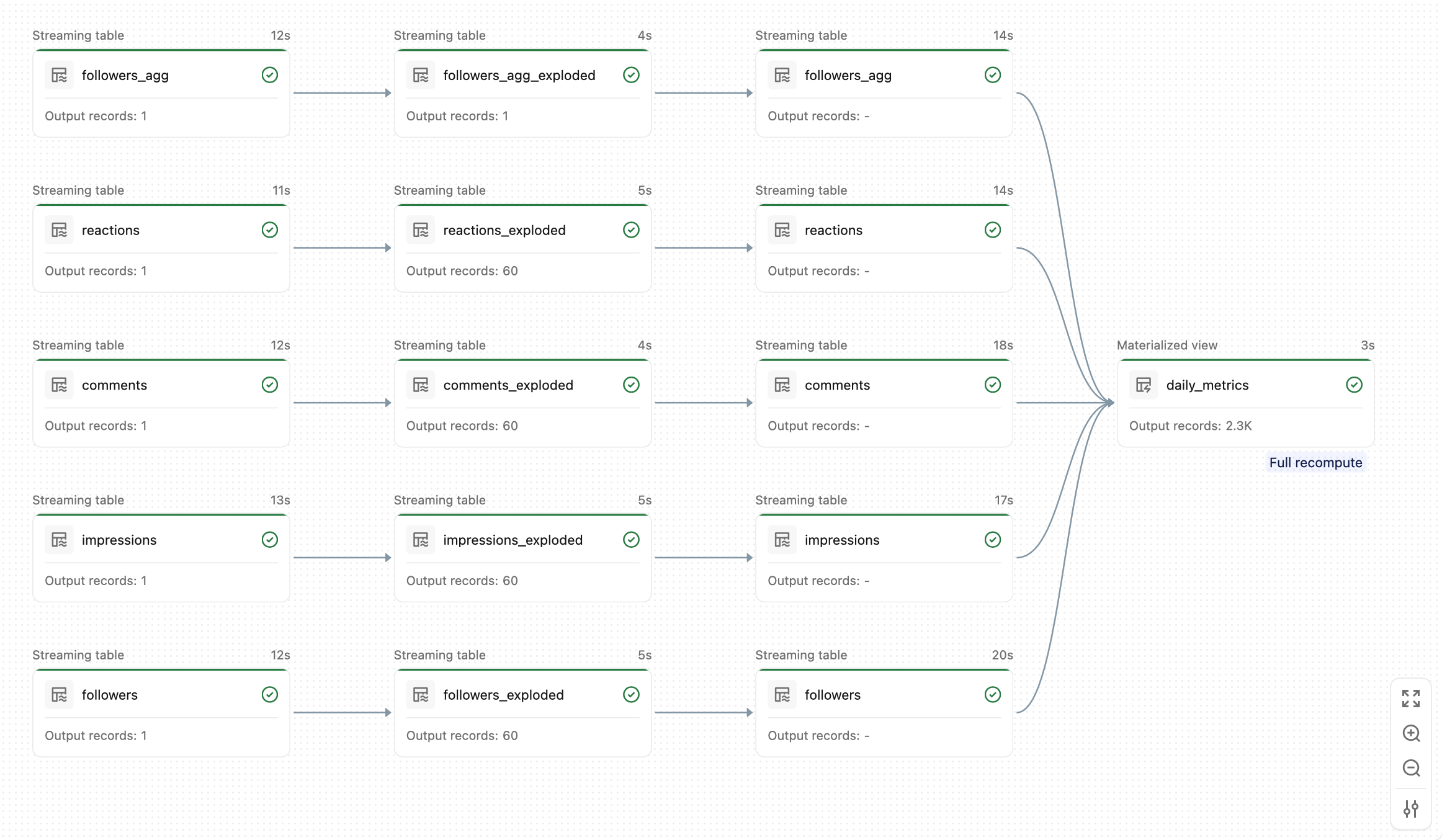
At this point you can deploy the bundle and test the pipeline. It should look something like this:

LinkedIn Medaillon Pipeline

Add the pipeline to the Job

What is missing is adding the pipeline to our job after the ingest task. Modify the jobs.yml so it looks like this:

resources:
  jobs:
    linkedin_medallion:
      name: linkedin-medallion
      schedule:
        quartz_cron_expression: "0 0 6 * * ?"
        timezone_id: "Europe/Berlin"
        pause_status: UNPAUSED

      parameters:
        - name: catalog
          default: ${var.catalog}
        - name: schema
          default: ${resources.schemas.bronze_linkedin.name}
        - name: volume
          default: ${resources.volumes.landing.name}
        - name: run_type
          default: ${var.run_type}

      run_as:
        service_principal_name: ${var.service_principal_app_id}

      tags:
        project: linkedin

      tasks:
        - task_key: ingest
          notebook_task:
            notebook_path: ../notebooks/ingest.ipynb
          environment_key: serverless

        - task_key: transform
          depends_on:
            - task_key: ingest
          pipeline_task:
            pipeline_id: ${resources.pipelines.linkedin_transform.id}

      environments:
        - environment_key: serverless
          spec:
            client: "4"

I added the transform task to the job referencing the pipeline we just set up. As a dependency, the ingest task is added to make sure the pipeline runs only after the ingestion is finished. Second, in order to automatically run this job every day, I added a schedule block that makes sure this pipeline runs every morning at 6 a.m. to pull the newest data from LinkedIn and process it into the Gold layer.

Job Structure with two tasks

The full code is available in the accompanying GitHub Repo. Click the Button below to view the repo.

What’s next

We are basically finished with the implementation of the pipeline. What comes next is actually using the data by creating a dashboard. We will also have a look at the cost of running this pipeline.

This will be covered in the fourth and last part of this series. It will be published on 2026/07/02